SVR

SVR (Support Vector Regression) solves the following optimization problem:

\[\min_{\mathbf{\beta} \in \mathbb{R}^d} \sum_{i=1}^{n} (|y_i - \mathbf{x}_i^\intercal \mathbf{\beta}| - \epsilon)_+ + \frac{\lambda}{2} \|\mathbf{\beta}\|^2\]

where \(\mathbf{x}_i \in \mathbb{R}^d\) is a feature vector, and \(y_i \in \mathbb{R}\) is a continuous response variable.

import numpy as np
import matplotlib.pyplot as plt
import pandas as pd
import seaborn as sns
import warnings
from sklearn.datasets import make_regression
from sklearn.preprocessing import StandardScaler

# Simulate data
np.random.seed(42)
scaler_svr = StandardScaler()

n, d = 10000, 5
X, y = make_regression(n_samples=n, n_features=d, noise=1.0)
X = scaler_svr.fit_transform(X)
X = np.hstack((X, np.ones((n, 1))))  # add intercept
y = y / y.std()

## solve SVR via `plqERM_Ridge`
from rehline import plqERM_Ridge

clf = plqERM_Ridge(loss={'name': 'svr', 'epsilon': 0.1}, C=1.0)
clf.fit(X=X, y=y)

plqERM_Ridge(loss={'epsilon': 0.1, 'name': 'svr'})

In a Jupyter environment, please rerun this cell to show the HTML representation or trust the notebook.
On GitHub, the HTML representation is unable to render, please try loading this page with nbviewer.org.

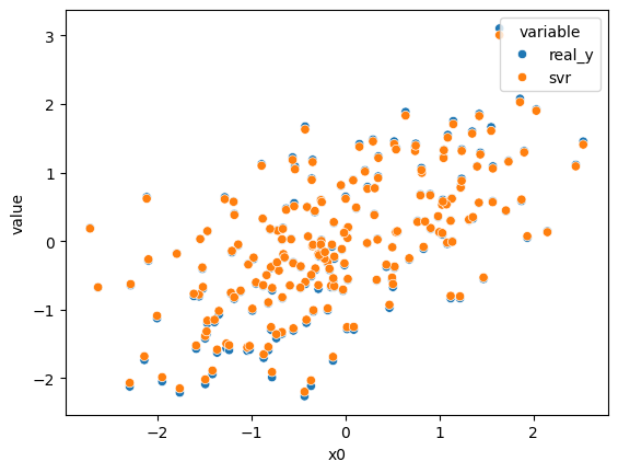
## plot SVR results
warnings.filterwarnings("ignore", "is_categorical_dtype")

n_sample = 200
X_sample, y_sample = X[:n_sample], y[:n_sample]
svr_sample = clf.decision_function(X_sample)

df = pd.DataFrame({'x0': X_sample[:,0], 'real_y': y_sample, 'svr': svr_sample})
df = df.melt(id_vars='x0')

sns.scatterplot(data=df, x='x0', y='value', hue='variable')
plt.show()