ReHLine with Scikit-Learn
ReHLine provides a versatile and powerful solver for empirical risk minimization problems with linear constraints. To make it even more accessible and easy to integrate into standard machine learning workflows, it now comes with a scikit-learn compatible estimator.
This means you can use ReHLine just like any other scikit-learn estimator, allowing you to seamlessly use it with scikit-learn’s rich ecosystem, including tools like Pipeline for building workflows and GridSearchCV for hyperparameter tuning.
This tutorial will guide you through the process of using the ReHLine scikit-learn estimator, from basic usage to advanced integration with scikit-learn’s powerful features.
Mathematical Formulation
The ReHLine solver addresses the following empirical risk minimization problem with a piecewise linear-quadratic (PLQ) loss, ridge regularization, and linear constraints. The objective function is:
- where:
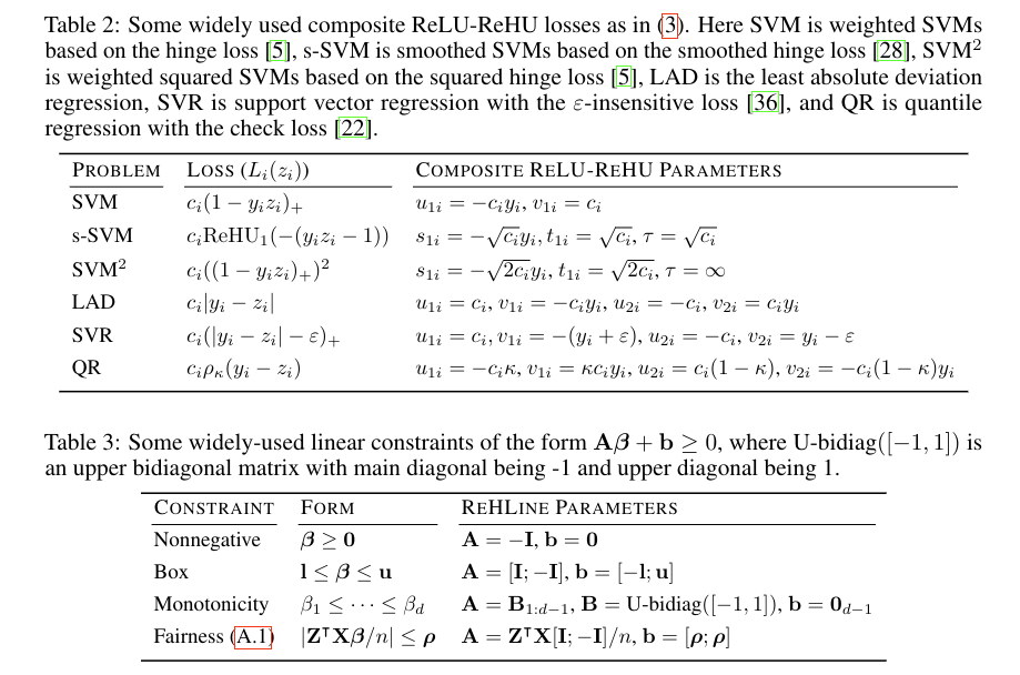
\(\text{PLQ}(\cdot, \cdot)\) is a convex piecewise linear-quadratic loss function. You can find built-in loss functions in the Loss section.
\(\mathbf{A}\) is a \(K \times d\) matrix and \(\mathbf{b}\) is a \(K\)-dimensional vector representing K linear constraints. See Constraints for more details.
For example, ReHLine supports the following loss functions and constraints:
Basic Usage
Here is a simple example of how to use the plq_Ridge_Classifier for a binary classification task. The estimator follows the standard scikit-learn API: fit(X, y) and predict(X).
import numpy as np
from sklearn.datasets import make_classification
from sklearn.model_selection import train_test_split
from rehline import plq_Ridge_Classifier

# Generate synthetic data
X, y = make_classification(n_samples=100, n_features=10, random_state=42)

# Split data into training and testing sets
X_train, X_test, y_train, y_test = train_test_split(X, y, test_size=0.2, random_state=42)

# Initialize and train the classifier
# We use the SVM loss as an example
clf = plq_Ridge_Classifier(loss={'name': 'svm'}, C=1.0)
clf.fit(X_train, y_train)

# Make predictions
y_pred = clf.predict(X_test)

# Print the accuracy
accuracy = clf.score(X_test, y_test)
print(f"Accuracy: {accuracy:.2f}")
Using ReHLine with Pipelines
You can easily integrate ReHLine estimators into scikit-learn Pipeline objects. This is useful for chaining preprocessing steps, such as feature scaling, with the ReHLine estimator.
from sklearn.pipeline import Pipeline
from sklearn.preprocessing import StandardScaler

# Create a pipeline with a scaler and the classifier
pipe = Pipeline([
    ('scaler', StandardScaler()),
    ('clf', plq_Ridge_Classifier(loss={'name': 'svm'}))
])

# The pipeline can be used as a single estimator
pipe.fit(X_train, y_train)
accuracy = pipe.score(X_test, y_test)
print(f"Pipeline Accuracy: {accuracy:.2f}")
Hyperparameter Tuning with GridSearchCV
The scikit-learn compatibility also allows you to use GridSearchCV to find the best hyperparameters for your ReHLine model.
from sklearn.model_selection import GridSearchCV

# Define the parameter grid to search
param_grid = {
    'clf__C': [0.1, 1.0, 10.0],
    'clf__loss': [{'name': 'svm'}, {'name': 'sSVM'}]
}

# Create the GridSearchCV object
grid_search = GridSearchCV(pipe, param_grid, cv=5)
grid_search.fit(X_train, y_train)

# Print the best parameters and score
print(f"Best Parameters: {grid_search.best_params_}")
print(f"Best CV Score: {grid_search.best_score_:.2f}")
Example
Emprical Risk Minimization
