Getting Started
This page provides a starter example to introduce users to the rehline package and showcase its primary features, facilitating exploration and familiarization.
To proceed, ensure that you have already installed rehline:
pip install rehline
rehline is a versatile solver for machine learning problems, particularly effective for Empirical Risk Minimization (ERM) with non-smooth objectives. We will use ERM as our starting example to demonstrate that:
Note
With rehline, you can easily transform different loss functions and add constraints to your ERM with no tears!
Let’s begin by generating a toy dataset and splitting it into training and test sets using scikit-learn’s make_regression.
# Import necessary libraries
import numpy as np
from sklearn.datasets import make_regression
from sklearn.model_selection import train_test_split
from sklearn.preprocessing import StandardScaler

np.random.seed(1024)
# Generate toy data
n, d = 1000, 5
scaler = StandardScaler()
X, y = make_regression(n_samples=n, n_features=d, noise=1.0)
# Normalize X and add intercept
X = scaler.fit_transform(X)
X = np.hstack((X, np.ones((n, 1))))

# Split data into training and test sets
X_train, X_test, y_train, y_test = train_test_split(X, y, test_size=50)
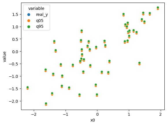
Quantile Regression
Next, let’s use rehline to fit a quantile regression (QR) at quantile level 0.95 (\(\kappa=0.95\)).
The ridge-regularized QR solves the following optimization problem:
where \(\rho_\kappa(u) = u \cdot (\kappa - \mathbf{1}(u < 0))\) is the check loss, \(x_i \in \mathbb{R}^d\) is a feature vector, and \(y_i \in \mathbb{R}\) is the response variable.
Since the check loss is a piecewise linear quadratic function (PLQ), it can be solved using rehline.plqERM_Ridge:
from rehline import plqERM_Ridge
# Define a QR estimator
clf = plqERM_Ridge(loss={'name': 'QR', 'qt': 0.95}, C=1.0)
clf.fit(X=X_train, y=y_train)
# Make predictions
q_predict = clf.decision_function(X_test)

# Plot results
import matplotlib.pyplot as plt
plt.scatter(x=X_test[:, 0], y=y_test, label='y_true')
plt.scatter(x=X_test[:, 0], y=q_predict, alpha=0.5, label='q_95')
plt.legend(loc="upper left")
plt.show()
Huber Regression
If you prefer Huber regression, it is also a PLQ function.
The ridge-regularized Huber minimization solves the following optimization problem:
where \(H_\kappa(\cdot)\) is the Huber loss defined as follows:
from rehline import plqERM_Ridge
# Define a Huber estimator
clf = plqERM_Ridge(loss={'name': 'huber', 'tau': 0.5}, C=1.0)
clf.fit(X=X_train, y=y_train)
# Make predictions
y_huber = clf.decision_function(X_test)

# Plot results
import matplotlib.pyplot as plt
plt.scatter(x=X_test[:, 0], y=y_test, label='y_true')
plt.scatter(x=X_test[:, 0], y=y_huber, alpha=0.5, label='y_huber')
plt.legend(loc="upper left")
plt.show()
Fairness Constraints
You have now learned that the fitted Huber regression requires a fairness constraint for the first feature \(\mathbf{X}_{1}\). Specifically, the correlation between the predicted \(\hat{Y}\) and \(\mathbf{X}_{1}\) must be less than tol=0.1, that is,
With rehline, you can easily add a fairness constraint to your ERM.
from rehline import plqERM_Ridge
from scipy.stats import pearsonr
# Define a Huber estimator with fairness constraint
clf = plqERM_Ridge(loss={'name': 'huber', 'tau': 0.5},
                   constraint=[{'name': 'fair', 'sen_idx': [0], 'tol_sen': 0.1}],
                   C=1.0,
                   max_iter=10000)
clf.fit(X=X_train, y=y_train)
# Make predictions
y_huber_fair = clf.decision_function(X_test)

# Plot results
import matplotlib.pyplot as plt
plt.scatter(x=X_test[:, 0], y=y_test, label='y_true')
plt.scatter(x=X_test[:, 0], y=y_huber, alpha=0.5, label='y_huber')
plt.scatter(x=X_test[:, 0], y=y_huber_fair, alpha=0.5, label='y_huber_fair')
plt.legend(loc="upper left")
plt.show()
Related Examples