Ridge Quantile Regression

The regularized quantile regression solves the following optimization problem:

\[\min_{\mathbf{\beta} \in \mathbb{R}^d} C \sum_{i=1}^n \rho_\kappa (y_i - \mathbf{x}_i^\top \mathbf{\beta}) + \frac{1}{2} \|\mathbf{\beta}\|^2,\]

where \(\rho_\kappa(u) = u \cdot (\kappa - \mathbf{1}(u < 0))\) is the check loss, \(\mathbf{x}_i \in \mathbb{R}^d\) is a feature vector, \(y_i \in \mathbb{R}\) is the response variable.

Note. Since the check loss is a plq function, we can optimize it using rehline.plq_Ridge_Regressor. Moreover, this wrapper adapts the plqERM_Ridge into a regressor, compatible with the scikit-learn API.

## install rehline
%pip install rehline -q

## simulate data
import numpy as np
from sklearn.datasets import make_regression
from sklearn.preprocessing import StandardScaler

scaler = StandardScaler()

n, d = 10000, 5
X, y = make_regression(n_samples=n, n_features=d, noise=1.0, random_state=42)
X = scaler.fit_transform(X)
y = y / y.std()

## solve QR with different `qt` via `plq_Ridge_Regressor`
from rehline import plq_Ridge_Regressor

clf5 = plq_Ridge_Regressor(loss={"name": "QR", "qt": 0.05}, C=10.0 / n)
clf5.fit(X=X, y=y)

clf95 = plq_Ridge_Regressor(loss={"name": "QR", "qt": 0.95}, C=10.0 / n)
clf95.fit(X=X, y=y)

plq_Ridge_Regressor(C=0.001, loss={'name': 'QR', 'qt': 0.95})

In a Jupyter environment, please rerun this cell to show the HTML representation or trust the notebook.
On GitHub, the HTML representation is unable to render, please try loading this page with nbviewer.org.

## plot QR results
import warnings

import matplotlib.pyplot as plt
import pandas as pd
import seaborn as sns

warnings.filterwarnings("ignore", "is_categorical_dtype")

n_sample = 50
X_sample, y_sample = X[:n_sample], y[:n_sample]
q05_sample = clf5.predict(X_sample)
q95_sample = clf95.predict(X_sample)

df = pd.DataFrame({"x0": X_sample[:, 0], "real_y": y_sample, "q05": q05_sample, "q95": q95_sample})
df = df.melt(id_vars="x0")

sns.scatterplot(data=df, x="x0", y="value", hue="variable").set_title("Ridge Quantile Regression")
plt.show()

With Pipeline

plq_Ridge_Regressor can be integrated into a scikit-learn Pipeline to streamline preprocessing including scaling.

## simulate data
from sklearn.datasets import make_regression
from sklearn.pipeline import Pipeline
from sklearn.preprocessing import StandardScaler

n, d = 10000, 5
X, y = make_regression(n_samples=n, n_features=d, noise=1.0, random_state=42)
y = y / y.std()

## solve QR with different `qt` via `plq_Ridge_Regressor`
from rehline import plq_Ridge_Regressor

pipe5 = Pipeline(
    [("scaler", StandardScaler()), ("reg", plq_Ridge_Regressor(loss={"name": "QR", "qt": 0.05}, C=10.0 / n))]
)
pipe5.fit(X=X, y=y)

pipe95 = Pipeline(
    [("scaler", StandardScaler()), ("reg", plq_Ridge_Regressor(loss={"name": "QR", "qt": 0.95}, C=10.0 / n))]
)
pipe95.fit(X=X, y=y)

Pipeline(steps=[('scaler', StandardScaler()),
                ('reg',
                 plq_Ridge_Regressor(C=0.001,
                                     loss={'name': 'QR', 'qt': 0.95}))])

In a Jupyter environment, please rerun this cell to show the HTML representation or trust the notebook.
On GitHub, the HTML representation is unable to render, please try loading this page with nbviewer.org.

## plot QR results
import warnings

import matplotlib.pyplot as plt
import pandas as pd
import seaborn as sns

warnings.filterwarnings("ignore", "is_categorical_dtype")

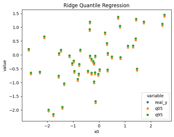
n_sample = 50
X_sample, y_sample = X[:n_sample], y[:n_sample]
q05_sample = pipe5.predict(X_sample)
q95_sample = pipe95.predict(X_sample)

df = pd.DataFrame({"x0": X_sample[:, 0], "real_y": y_sample, "q05": q05_sample, "q95": q95_sample})
df = df.melt(id_vars="x0")

sns.scatterplot(data=df, x="x0", y="value", hue="variable").set_title("Ridge Quantile Regression")
plt.show()

Hyperparameter Tuning with GridSearchCV

Due to its compatibility with the scikit-learn API, GridSearchCV can be applied to determine the optimal hyperparameters for the ReHLine model.

import warnings

from sklearn.metrics import make_scorer, mean_pinball_loss
from sklearn.model_selection import GridSearchCV

warnings.filterwarnings("ignore")

# Define the parameter grid to search
param_grid = {"reg__C": [100.0 / n, 10.0 / n, 1.0 / n]}

# Use negative pinball
scorer05 = make_scorer(mean_pinball_loss, alpha=0.05, greater_is_better=False)
scorer95 = make_scorer(mean_pinball_loss, alpha=0.95, greater_is_better=False)

# Create the GridSearchCV objects
grid_search5 = GridSearchCV(pipe5, param_grid, cv=5, scoring=scorer05)
grid_search95 = GridSearchCV(pipe95, param_grid, cv=5, scoring=scorer95)

grid_search5.fit(X, y)
grid_search95.fit(X, y)

# Print the best parameters and scores
print(f"Best Parameters (qt=0.05): {grid_search5.best_params_}")
print(f"Best CV Score (qt=0.05): {-grid_search5.best_score_:.4f}")

print(f"Best Parameters (qt=0.95): {grid_search95.best_params_}")
print(f"Best CV Score (qt=0.95): {-grid_search95.best_score_:.4f}")

Best Parameters (qt=0.05): {'reg__C': 0.01}
Best CV Score (qt=0.05): 0.0008
Best Parameters (qt=0.95): {'reg__C': 0.01}
Best CV Score (qt=0.95): 0.0008

import warnings

import matplotlib.pyplot as plt
import pandas as pd
import seaborn as sns

warnings.filterwarnings("ignore", "is_categorical_dtype")
warnings.filterwarnings("ignore", "use_inf_as_na")

n_sample = 50
X_sample, y_sample = X[:n_sample], y[:n_sample]
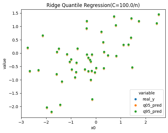
q05_sample = grid_search5.predict(X_sample)
q95_sample = grid_search95.predict(X_sample)

df = pd.DataFrame({"x0": X_sample[:, 0], "real_y": y_sample, "q05_pred": q05_sample, "q95_pred": q95_sample})
df = df.melt(id_vars="x0")

sns.scatterplot(data=df, x="x0", y="value", hue="variable").set_title("Ridge Quantile Regression(C=100.0/n)")
plt.show()