Path solution
We use the simulated data together with different loss function and constraint to solve the optimization problem. Meanwhile, a plot of path solution concerning different C values will be displayed.
All the following test used
warm-starttechnique.
SVM with nonnegative constraint
[ ]:
## generate data
import numpy as np

np.random.seed(1042)
n, d, C = 1000, 5, 0.5
X = np.random.randn(n, d)
beta0 = np.random.randn(d)
y = np.sign(X.dot(beta0) + np.random.randn(n))
[ ]:
## define loss function
loss = {"name": "SVM"}

## define constraint
constraint = [{"name": "nonnegative"}]

## define value of Cs
Cs = np.logspace(-5, 3, 20)
[ ]:
## solve SVM and show path solution via `plqERM_Ridge_path_sol`
from rehline import plqERM_Ridge_path_sol

Cs, times, n_iters, losses, norms, coefs = plqERM_Ridge_path_sol(
    X,
    y,
    loss=loss,
    Cs=Cs,
    max_iter=200000,
    tol=1e-4,
    verbose=2,
    warm_start=True,
    constraint=constraint,
    return_time=True,
)
PLQ ERM Path Solution Results
==========================================================================================
C Value        Iterations     Time (s)            Loss                L2 Norm
------------------------------------------------------------------------------------------
1e-05          3              0.001964            995.663000          0.006600
2.637e-05      1              0.000679            988.564800          0.017400
6.952e-05      1              0.000593            969.850000          0.045800
0.0001833      1              0.000593            920.509600          0.120700
0.0004833      2              0.000522            791.465800          0.316700
0.001274       8              0.000578            634.164300          0.590300
0.00336        13             0.000771            541.042400          0.860000
0.008859       16             0.000767            495.021900          1.113600
0.02336        48             0.000763            474.343400          1.346800
0.06158        286            0.004387            463.425100          1.612800
0.1624         68             0.000982            461.875400          1.711300
0.4281         676            0.001370            461.471000          1.776600
1.129          1813           0.002026            461.420300          1.829500
2.976          2068           0.002215            461.403400          1.835800
7.848          2639           0.002831            461.438100          1.841200
20.69          2826           0.003130            461.454300          1.844800
54.56          3376           0.004949            461.456300          1.844700
143.8          3429           0.005815            461.450600          1.844700
379.3          3429           0.019599            461.450600          1.844700
1000           3429           0.004155            461.450600          1.844700
==========================================================================================
Total Time  0.058876 sec
Avg Time/Iter0.000002 sec
==========================================================================================

SVM with fair constraint
[ ]:
## simulate data
import numpy as np
from sklearn.datasets import make_classification
from sklearn.preprocessing import StandardScaler

scaler = StandardScaler()

n, d = 10000, 5
X, y = make_classification(n_samples=n, n_features=d, n_redundant=0)
## convert y to +1/-1
y = 2 * y - 1
X = scaler.fit_transform(X)
[ ]:
## we take the first column of X as sensetive features, and tol is 0.1
sen_idx = [0]
tol_sen = 0.1
# define constraint
constraint = [{"name": "fair", "sen_idx": sen_idx, "tol_sen": tol_sen}]
# define loss function
loss = {"name": "SVM"}
# define value of Cs
Cs = np.logspace(-4, 2, 30)
[ ]:
## solve FairSVM and show path solution via `plqERM_Ridge_path_sol`
from rehline import plqERM_Ridge_path_sol

Cs, times, n_iters, losses, norms, coefs = plqERM_Ridge_path_sol(
    X,
    y,
    loss=loss,
    Cs=Cs,
    max_iter=2000000,
    tol=1e-4,
    verbose=2,
    warm_start=True,
    constraint=constraint,
    return_time=True,
)
PLQ ERM Path Solution Results
==========================================================================================
C Value        Iterations     Time (s)            Loss                L2 Norm
------------------------------------------------------------------------------------------
0.0001         12             0.003890            5972.764500         0.578600
0.000161       3              0.002714            5240.628500         0.721300
0.0002593      3              0.002834            4681.713900         0.865200
0.0004175      4              0.002385            4289.990700         1.002700
0.0006723      3              0.002681            3969.397000         1.159200
0.001083       4              0.002964            3761.419300         1.302600
0.001743       5              0.002581            3596.565300         1.466700
0.002807       20             0.003389            3486.067800         1.623000
0.00452        11             0.003425            3411.601500         1.777500
0.007279       20             0.003167            3366.919700         1.916000
0.01172        30             0.004878            3339.163800         2.043100
0.01887        33             0.003196            3324.690900         2.144600
0.03039        114            0.003661            3318.217200         2.216600
0.04894        265            0.007217            3315.451400         2.267100
0.0788         159            0.004054            3313.904600         2.310200
0.1269         835            0.008838            3313.253500         2.339800
0.2043         1103           0.013295            3312.989100         2.359600
0.329          713            0.016122            3312.932600         2.367300
0.5298         1901           0.023764            3312.909400         2.374600
0.8532         994            0.005804            3312.905000         2.378000
1.374          2094           0.008422            3312.905300         2.381100
2.212          3589           0.036307            3312.906200         2.381200
3.562          1758           0.028580            3312.908800         2.383200
5.736          2506           0.040888            3312.908800         2.383200
9.237          2479           0.043123            3312.908700         2.383200
14.87          2479           0.046010            3312.908700         2.383200
23.95          2479           0.042148            3312.908700         2.383200
38.57          2479           0.039667            3312.908700         2.383200
62.1           2479           0.040740            3312.908700         2.383200
100            2479           0.041395            3312.908700         2.383200
==========================================================================================
Total Time  0.488429 sec
Avg Time/Iter0.000016 sec
==========================================================================================

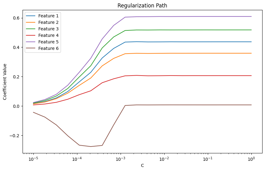
Quantile regression without any constraint
[ ]:
## simulate data
import numpy as np
from sklearn.datasets import make_regression
from sklearn.preprocessing import StandardScaler

scaler = StandardScaler()

n, d = 10000, 5
X, y = make_regression(n_samples=n, n_features=d, noise=1.0)
X = scaler.fit_transform(X)
## add intercept
X = np.hstack((X, np.ones((n, 1))))
y = y / y.std()
[ ]:
## define loss function
loss = {"name": "QR", "qt": 0.05}

# define value of Cs
Cs = np.logspace(-5, 0, 20)
[ ]:
## solve QR and show path solution via `plqERM_Ridge_path_sol`
from rehline import plqERM_Ridge_path_sol

Cs, times, n_iters, losses, norms, coefs = plqERM_Ridge_path_sol(
    X, y, loss=loss, Cs=Cs, max_iter=10000, tol=1e-4, verbose=2, warm_start=True, return_time=True
)
PLQ ERM Path Solution Results
==========================================================================================
C Value        Iterations     Time (s)            Loss                L2 Norm
------------------------------------------------------------------------------------------
1e-05          0              0.004709            3543.001300         0.058100
1.833e-05      0              0.003891            3277.611200         0.104300
3.36e-05       0              0.003566            2835.021100         0.183600
6.158e-05      0              0.003944            2176.310400         0.308200
0.0001129      0              0.003700            1435.686300         0.464300
0.0002069      0              0.003558            905.373700          0.596400
0.0003793      3              0.007558            286.819900          0.801800
0.0006952      2              0.006340            101.797200          0.911600
0.001274       2              0.006275            10.476100           0.994100
0.002336       2              0.006263            7.682400            1.000500
0.004281       7              0.012215            7.705400            0.998900
0.007848       15             0.019309            7.286400            1.000500
0.01438        31             0.033054            7.254300            1.000800
0.02637        121            0.080112            7.214700            1.000800
0.04833        238            0.153759            7.209100            1.001000
0.08859        256            0.156395            7.209400            1.001100
0.1624         412            0.224236            7.207500            1.001100
0.2976         375            0.227330            7.208600            1.001200
0.5456         349            0.215738            7.208100            1.001200
1              301            0.176951            7.208100            1.001200
==========================================================================================
Total Time  1.349375 sec
Avg Time/Iter0.000638 sec
==========================================================================================
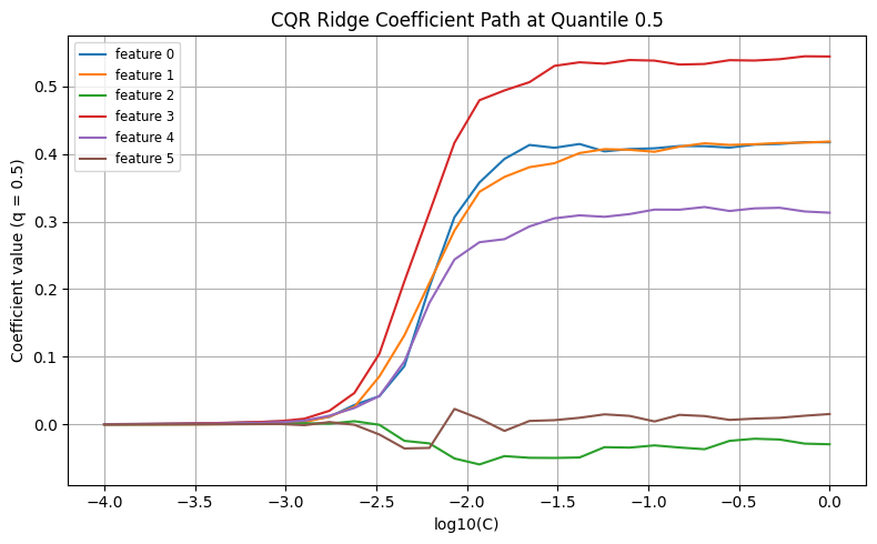
Ridge Composite Quantile Regression
[2]:
## simulate data
import matplotlib.pyplot as plt
import numpy as np
from sklearn.datasets import make_friedman1
from sklearn.preprocessing import StandardScaler

X, y = make_friedman1(n_samples=500, n_features=6, noise=1.0, random_state=42)
X = StandardScaler().fit_transform(X)
y = y / y.std()
[3]:
## define the quantiles
quantiles = [0.1, 0.5, 0.9]
## define the value of Cs
Cs = np.logspace(-4, 0, 30)
[5]:
## solve the Ridge Composite Quantile Regression
from rehline import CQR_Ridge_path_sol

Cs, models, coefs, intercepts, fit_times = CQR_Ridge_path_sol(
    X, y, quantiles=quantiles, Cs=Cs, max_iter=100000, tol=1e-4, verbose=0, shrink=1, warm_start=True, return_time=True
)
[6]:
target_index = 1
log_Cs = np.log10(Cs)

## Coefficient path plot
# all three quantiles share the same coefficient
# here only plot path solution for one quantile
plt.figure(figsize=(8, 5))
for j in range(coefs.shape[2]):
    plt.plot(log_Cs, coefs[:, target_index, j], label=f"feature {j}")
plt.xlabel("log10(C)")
plt.ylabel(f"Coefficient value (q = {quantiles[target_index]})")
plt.title(f"CQR Ridge Coefficient Path at Quantile {quantiles[target_index]}")
plt.grid(True)
plt.legend(loc="best", fontsize="small")
plt.tight_layout()
plt.show()
[7]:
## Intercept path plot
plt.figure(figsize=(8, 5))
n_quantiles = intercepts.shape[1]

for q in range(n_quantiles):
    plt.plot(log_Cs, intercepts[:, q], marker="o", label=f"Intercept (q={quantiles[q]:.2f})")

plt.xlabel("log10(C)")
plt.ylabel("Intercept Value")
plt.title("CQR Ridge Intercept Path Across Quantiles")
plt.grid(True)
plt.legend()
plt.tight_layout()
plt.show()
