Multi-class Classification Support

PLQ_Ridge_Classifier extends binary PLQ-ERM to multi-class problems via the multi_class parameter, supporting two standard decomposition strategies.

One-vs-Rest (OvR) fits \(K\) binary classifiers, one per class, each trained on the full dataset with relabelled targets (\(+1\) for the class, \(-1\) for all others). Prediction selects the class with the highest decision score:

\[\widehat{y} = \arg\max_{k \in \{1, \dots, K\}} f_k(\mathbf{x})\]

One-vs-One (OvO) fits \(\binom{K}{2}\) binary classifiers, one per class pair \((i, j)\), each trained only on samples belonging to those two classes. Prediction uses majority voting across all pairwise classifiers:

\[\widehat{y} = \arg\max_{k \in \{1, \dots, K\}} \sum_{j \neq k} \mathbf{1}\bigl[f_{kj}(\mathbf{x}) > 0\bigr]\]

In both cases, each binary sub-problem is solved by a standard PLQ_Ridge_Classifier with the same loss, regularizer, and solver settings passed to the parent estimator.

import matplotlib.pyplot as plt
from sklearn.datasets import make_classification
from sklearn.decomposition import PCA
from sklearn.metrics import ConfusionMatrixDisplay, accuracy_score, confusion_matrix
from sklearn.model_selection import train_test_split

from rehline import plq_Ridge_Classifier

# generate data
X_mc, y_mc = make_classification(
    n_samples=10000, n_features=20, n_informative=10, n_classes=4, n_clusters_per_class=1, random_state=42
)
X_train, X_test, y_train, y_test = train_test_split(X_mc, y_mc, test_size=0.2, random_state=42)

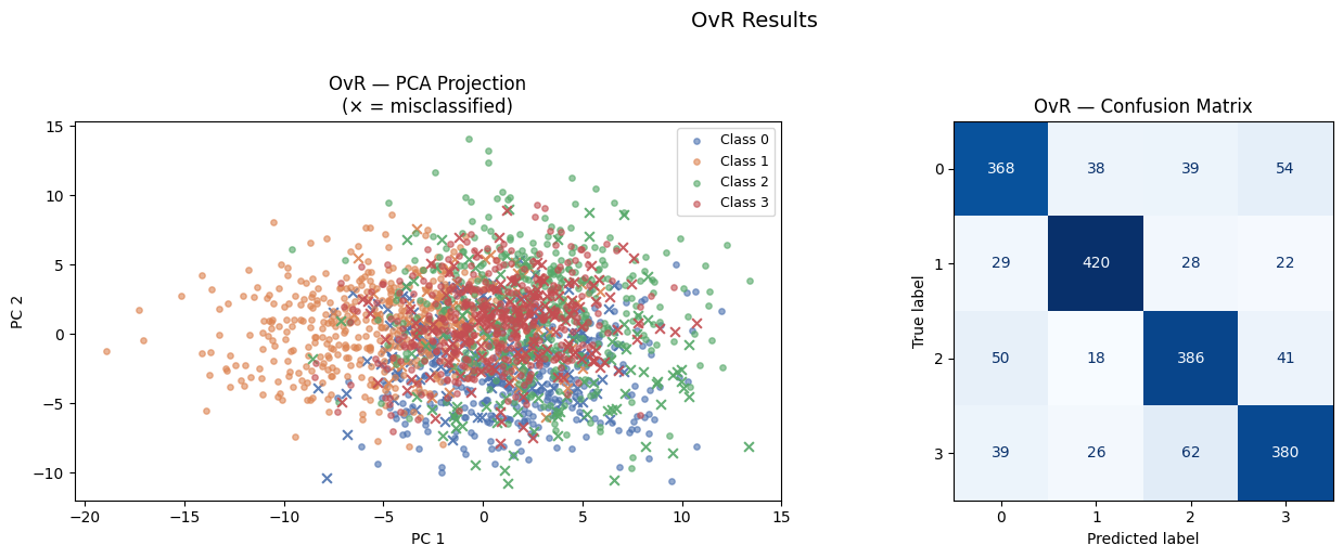
One-vs-Rest (OvR)

In OvR, we train \(K\) binary classifiers, one per class. Classifier \(k\) learns to distinguish class \(k\) from all other classes. The final prediction selects the class whose classifier reports the highest decision score:

\[\widehat{y} \;=\; \arg\max_{k \in \{1, \dots, K\}} f_k(\mathbf{x})\]

where \(f_k(\mathbf{x})\) is the signed distance from \(\mathbf{x}\) to the decision boundary of classifier \(k\).

# predict using ovr method
plq_ovr = plq_Ridge_Classifier(
    loss={"name": "svm"},
    C=1.0,
    fit_intercept=True,
    max_iter=50000,
    multi_class="ovr",
)
plq_ovr.fit(X_train, y_train)

y_pred = plq_ovr.predict(X_test)
print(f"plq OvR accuracy: {accuracy_score(y_test, y_pred):.4f}")

plq OvR accuracy: 0.7770

# results visualization
pca = PCA(n_components=2, random_state=42)
X_test_2d = pca.fit_transform(X_test)

fig, axes = plt.subplots(1, 2, figsize=(14, 5))

colors = ["#4C72B0", "#DD8452", "#55A868", "#C44E52"]
ax = axes[0]
for k, cls in enumerate(plq_ovr.classes_):
    mask_correct = (y_test == cls) & (y_pred == cls)
    mask_wrong = (y_test == cls) & (y_pred != cls)
    ax.scatter(
        X_test_2d[mask_correct, 0], X_test_2d[mask_correct, 1], c=colors[k], label=f"Class {cls}", s=15, alpha=0.6
    )
    ax.scatter(X_test_2d[mask_wrong, 0], X_test_2d[mask_wrong, 1], c=colors[k], marker="x", s=40, alpha=0.9)
ax.set_title("OvR — PCA Projection\n(× = misclassified)", fontsize=12)
ax.set_xlabel("PC 1")
ax.set_ylabel("PC 2")
ax.legend(fontsize=9)

cm = confusion_matrix(y_test, y_pred)
ConfusionMatrixDisplay(cm, display_labels=plq_ovr.classes_).plot(ax=axes[1], colorbar=False, cmap="Blues")
axes[1].set_title("OvR — Confusion Matrix", fontsize=12)

plt.suptitle("OvR Results", fontsize=14, y=1.02)
plt.tight_layout()
plt.show()

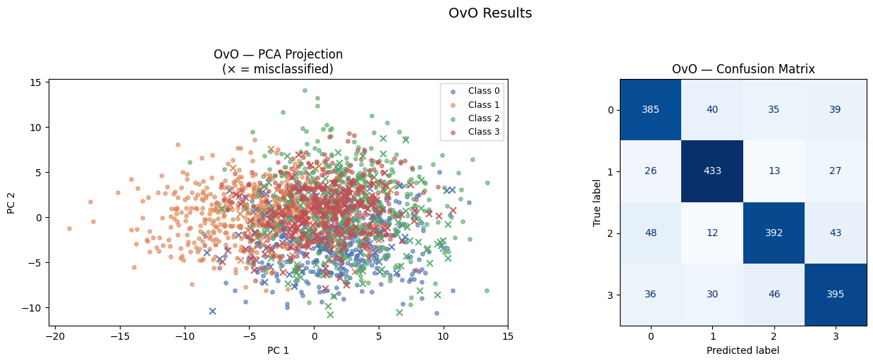
One-vs-One (OvO)

In OvO, we train \(\binom{K}{2}\) binary classifiers, one for each pair of classes \((i, j)\). Each classifier \(f_{ij}\) votes for either class \(i\) or class \(j\). The final prediction is the class that receives the most votes:

\[\widehat{y} = \arg\max_{k \in \{1, \dots, K\}} \sum_{j \neq k} \mathbf{1}\bigl[f_{kj}(\mathbf{x}) > 0\bigr]\]

where \(\mathbf{1}[\cdot]\) is the indicator function, and \(f_{kj}(\mathbf{x}) > 0\) means classifier \((k, j)\) votes for class \(k\).

# predict using ovo method
plq_ovo = plq_Ridge_Classifier(
    loss={"name": "svm"},
    C=0.7,
    fit_intercept=True,
    max_iter=50000,
    multi_class="ovo",
)
plq_ovo.fit(X_train, y_train)
y_pred = plq_ovo.predict(X_test)

print(f"plq OvO accuracy: {accuracy_score(y_test, y_pred):.4f}")

plq OvO accuracy: 0.8025

# results visualization
fig, axes = plt.subplots(1, 2, figsize=(14, 5))

ax = axes[0]
for k, cls in enumerate(plq_ovo.classes_):
    mask_correct = (y_test == cls) & (y_pred == cls)
    mask_wrong = (y_test == cls) & (y_pred != cls)
    ax.scatter(
        X_test_2d[mask_correct, 0], X_test_2d[mask_correct, 1], c=colors[k], label=f"Class {cls}", s=15, alpha=0.6
    )
    ax.scatter(X_test_2d[mask_wrong, 0], X_test_2d[mask_wrong, 1], c=colors[k], marker="x", s=40, alpha=0.9)
ax.set_title("OvO — PCA Projection\n(× = misclassified)", fontsize=12)
ax.set_xlabel("PC 1")
ax.set_ylabel("PC 2")
ax.legend(fontsize=9)

cm = confusion_matrix(y_test, y_pred)
ConfusionMatrixDisplay(cm, display_labels=plq_ovo.classes_).plot(ax=axes[1], colorbar=False, cmap="Blues")
axes[1].set_title("OvO — Confusion Matrix", fontsize=12)

plt.suptitle("OvO Results", fontsize=14, y=1.02)
plt.tight_layout()
plt.show()