Ridge Composite Quantile Regression

The regularized composite quantile regression solves the following optimization problem:

\[min_{\beta \in \mathbb{R}^{d}, \alpha \in \mathbb{R}^{K}} \ C \sum_{k=1}^K \sum_{i=1}^n \rho_\kappa ( y_i - x^\intercal_i \beta - \alpha_k) + \frac{1}{2} (\| \beta \|^2 + \| \alpha \|^2),\]

where \(\alpha_k\) is the intercept associated with k-th quantile, \(\rho_\kappa(u) = u\cdot(\kappa - \mathbf{1}(u < 0))\) is the check loss, \(x_i \in \mathbb{R}^d\) is a feature vector, \(y_i \in \mathbb{R}\) is the response variable.

## simulate data
from sklearn.datasets import make_regression
from sklearn.preprocessing import StandardScaler

scaler = StandardScaler()

n, d = 1000, 1
X, y, coef = make_regression(n_samples=n, n_features=d, noise=50.0, coef=True)
X = scaler.fit_transform(X)
y = y / y.std()

## fit model
from rehline import CQR_Ridge

cqr = CQR_Ridge(quantiles=[0.05, 0.5, 0.95])
cqr.fit(X, y)
y_pred = cqr.predict(X)  # 3 columns, each represents the prediction for a quantile

## plot QR results
import matplotlib.pyplot as plt
import pandas as pd
import seaborn as sns

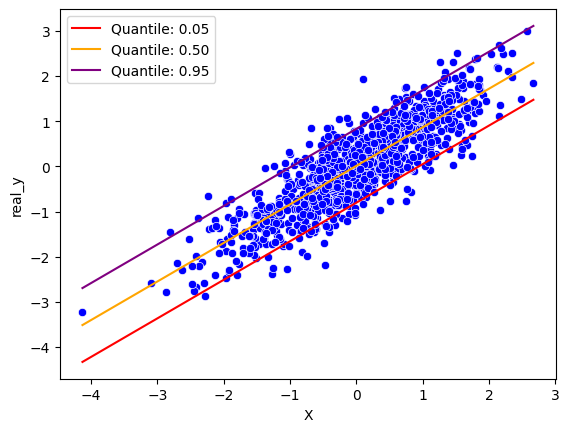
df = pd.DataFrame({"X": X.squeeze(), "real_y": y, "q05": y_pred[:, 0], "q50": y_pred[:, 1], "q95": y_pred[:, 2]})

## scatter plot of the data
sns.scatterplot(df, x="X", y="real_y", color="blue")

## plot the quantile regression lines
sns.lineplot(df, x="X", y="q05", color="red", label="Quantile: 0.05")
sns.lineplot(df, x="X", y="q50", color="orange", label="Quantile: 0.50")
sns.lineplot(df, x="X", y="q95", color="purple", label="Quantile: 0.95")
plt.show()