Monotonic SVM

The Monotonic SVM solves the following optimization problem:

\[\min_{\mathbf{\beta} \in \mathbb{R}^d} C\sum_{i=1}^n (1 - y_i \mathbf{\beta}^\intercal \mathbf{x}_i)_+ + \frac{1}{2} \|\mathbf{\beta}\|_2^2,\]

\[\text{subject to} \quad \beta_j \le \beta_{j+1} \quad \forall j \in \{1, \dots, d-1\} \quad (\text{Increasing})\]

\[\text{or} \quad \beta_j \ge \beta_{j+1} \quad \forall j \in \{1, \dots, d-1\} \quad (\text{Decreasing})\]

where:

• \(\mathbf{x}_i \in \mathbb{R}^d\) is a feature vector

• \(y_i \in \{-1, 1\}\) is a binary label

• \(\beta_j\) represents the \(j\)-th component of the coefficient vector \(\mathbf{\beta}\)

The monotonicity constraints ensure that the learned coefficients \(\beta\) follow a strictly non-decreasing or non-increasing order, useful when incorporating prior domain knowledge.

Note. Since the hinge loss is a plq function and the monotonicity constraints are purely linear (e.g., \(\beta_j - \beta_{j+1} \le 0\)), we can optimize it using rehline.plq_Ridge_Classifier.

## install rehline
%pip install rehline -q

## simulate data
from sklearn.datasets import make_classification
from sklearn.preprocessing import StandardScaler
import numpy as np

scaler = StandardScaler()

n, d = 10000, 5
X, y = make_classification(n_samples=n, n_features=d, n_redundant=0, random_state=42)
y = 2*y - 1
X = scaler.fit_transform(X)

SVM as baseline

## we first run a SVM
from rehline import plq_Ridge_Classifier

clf = plq_Ridge_Classifier(loss={'name': 'svm'}, C=0.001, max_iter=10000)
clf.fit(X=X, y=y)

plq_Ridge_Classifier(C=0.001, loss={'name': 'svm'}, max_iter=10000)

In a Jupyter environment, please rerun this cell to show the HTML representation or trust the notebook.
On GitHub, the HTML representation is unable to render, please try loading this page with nbviewer.org.

Monotonic constraint

## solve SVM with Monotonicity Constraint via `plq_Ridge_Classifier`
from rehline import plq_Ridge_Classifier
mclf = plq_Ridge_Classifier(
    loss={'name': 'svm'},
    constraint = [{'name': 'monotonic', 'decreasing': True}],
    C=0.001,
    max_iter=10000
)
mclf.fit(X=X, y=y)

plq_Ridge_Classifier(C=0.001,
                     constraint=[{'decreasing': True, 'name': 'monotonic'}],
                     loss={'name': 'svm'}, max_iter=10000)

In a Jupyter environment, please rerun this cell to show the HTML representation or trust the notebook.
On GitHub, the HTML representation is unable to render, please try loading this page with nbviewer.org.

Results

import pandas as pd

## score
score  = clf.decision_function(X)
mscore = mclf.decision_function(X)

svm_perf  = clf.score(X, y)
msvm_perf = mclf.score(X, y)

## Create a pandas DataFrame to store the results
results = pd.DataFrame({
    'Model': ['Standard SVM', 'Monotonic SVM'],
    'Performance': [svm_perf, msvm_perf]
})

## Print the results as a table
print(results.to_string(index=False))

        Model  Performance
 Standard SVM       0.8870
Monotonic SVM       0.7332

## Visualize the feature coefficients
import seaborn as sns
import matplotlib.pyplot as plt

df_coef = pd.DataFrame({
    'Feature Index': range(len(clf.coef_.flatten())),
    'SVM': clf.coef_.flatten(),
    'Monotonic SVM': mclf.coef_.flatten()
})

fig, axes = plt.subplots(1, 2, figsize=(14, 5), sharey=True)
sns.barplot(data=df_coef, x="Feature Index", y="SVM", ax=axes[0], color='#FFE4E1', edgecolor='black')
axes[0].axhline(0, color='black', linewidth=1)
axes[0].set_yscale('symlog', linthresh=0.005)
axes[0].set_title("SVM Coefficients (symlog)")

sns.barplot(data=df_coef, x="Feature Index", y="Monotonic SVM", color='#8A8293', ax=axes[1], edgecolor='black')
axes[1].axhline(0, color='black', linewidth=1)
axes[1].set_yscale('symlog', linthresh=0.005)
axes[1].set_title("Monotonic SVM Coefficients (symlog)")
plt.tight_layout()
plt.show()

## Print the results of monotonic constraint
np.set_printoptions(precision=5, suppress=True)
print("\nCoefficients (monotonic decreasing):")
print(mclf.coef_)
print("Monotonic descreasing satisfied:",
      np.all(mclf.coef_[:-1] >= mclf.coef_[1:]))

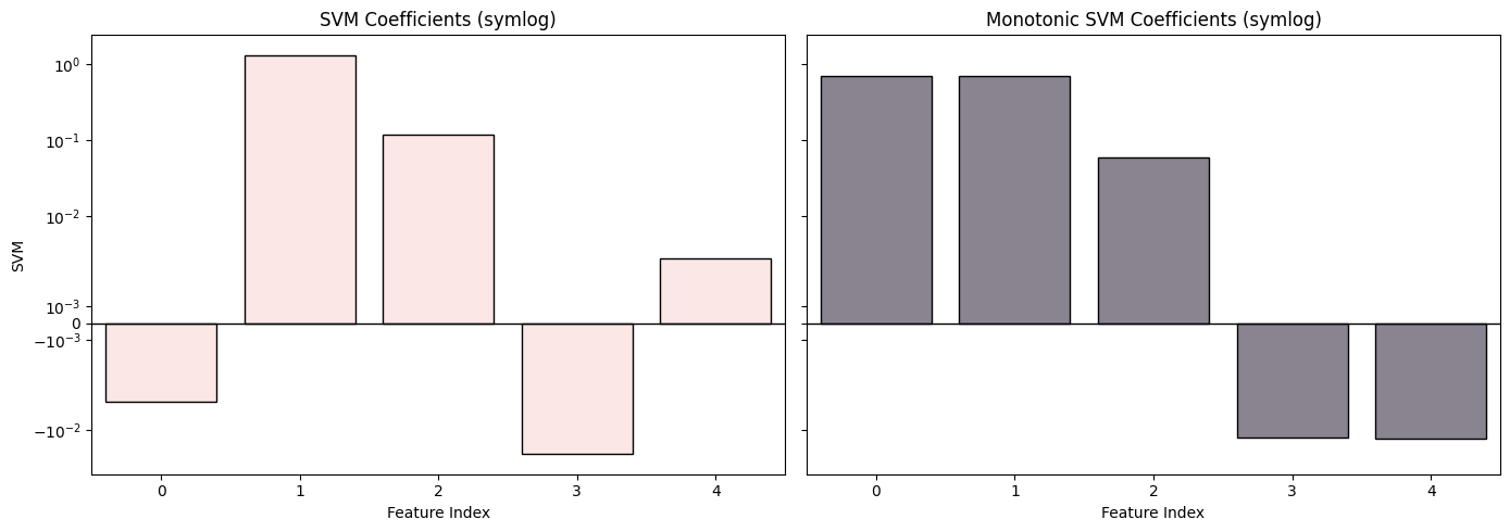
Coefficients (monotonic decreasing):
[ 0.6899   0.68989  0.05962 -0.0126  -0.01276]
Monotonic descreasing satisfied: True

import warnings
warnings.filterwarnings("ignore", "is_categorical_dtype")
warnings.filterwarnings("ignore", "use_inf_as_na")

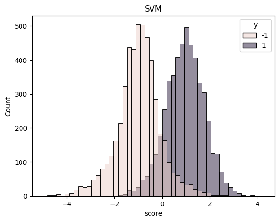
df = pd.DataFrame({'score': score, 'mscore': mscore, 'y': y})

sns.histplot(df, x="score", hue="y").set_title("SVM")
plt.show()
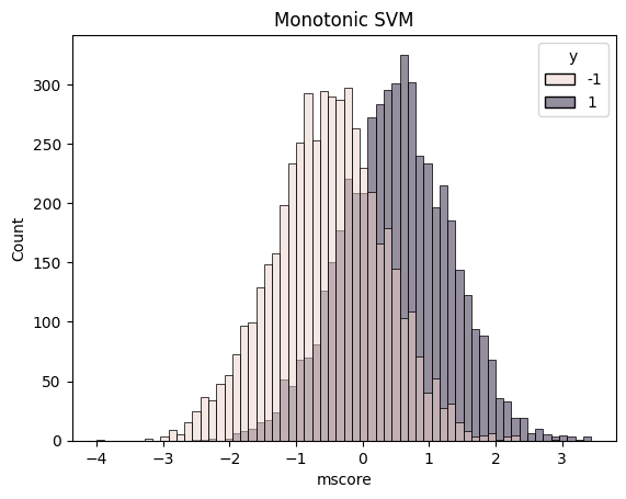
sns.histplot(df, x="mscore", hue="y").set_title("Monotonic SVM")
plt.show()