Compare SVM Losses with GridSearchCV

Due to its compatibility with the scikit-learn API, GridSearchCV can be used to compare SVM, Smooth SVM, and Squared SVM losses under a unified pipeline, identify the best loss, and select its optimal hyperparameter.

## install rehline
%pip install rehline -q

## set up plotting style
import seaborn as sns
import matplotlib.pyplot as plt
custom_palette = ['#FFE4E1', '#3D325C']
sns.set_palette(custom_palette)

## simulate data
from sklearn.datasets import make_classification
import numpy as np

n, d = 10000, 5
X, y = make_classification(n_samples=n, n_features=d, random_state=42)
y = 2*y - 1

## compare SVM losses via GridSearchCV
from sklearn.pipeline import Pipeline
from sklearn.preprocessing import StandardScaler
from rehline import plq_Ridge_Classifier
from sklearn.model_selection import GridSearchCV
import warnings
warnings.filterwarnings("ignore")

pipe = Pipeline([
    ('scaler', StandardScaler()),
    ('clf', plq_Ridge_Classifier(loss={'name': 'svm'}))
])

# Define the parameter grid to search
param_grid = {
    'clf__C': [0.1, 1.0, 10.0],
    'clf__loss': [{'name': 'svm'}, {'name': 'sSVM'}, {'name': 'squared SVM'}]
}

# Create the GridSearchCV object
grid_search = GridSearchCV(pipe, param_grid, cv=5)
grid_search.fit(X, y)

GridSearchCV(cv=5,
             estimator=Pipeline(steps=[('scaler', StandardScaler()),
                                       ('clf',
                                        plq_Ridge_Classifier(loss={'name': 'svm'}))]),
             param_grid={'clf__C': [0.1, 1.0, 10.0],
                         'clf__loss': [{'name': 'svm'}, {'name': 'sSVM'},
                                       {'name': 'squared SVM'}]})

In a Jupyter environment, please rerun this cell to show the HTML representation or trust the notebook.
On GitHub, the HTML representation is unable to render, please try loading this page with nbviewer.org.

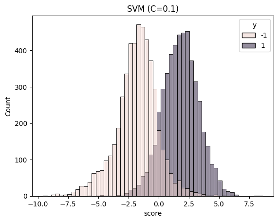
# Print the best loss function and score
print(f"Overall Best Params: {grid_search.best_params_}")
print(f"Overall Best Score:  {grid_search.best_score_:.4f}")

Overall Best Params: {'clf__C': 0.1, 'clf__loss': {'name': 'svm'}}
Overall Best Score:  0.8922

import seaborn as sns
import pandas as pd
import warnings
import matplotlib.pyplot as plt
warnings.filterwarnings("ignore", "is_categorical_dtype")
warnings.filterwarnings("ignore", "use_inf_as_na")

score = grid_search.decision_function(X)
df = pd.DataFrame({'score': score, 'y': y})
sns.histplot(data=df, x="score", hue="y").set_title("SVM (C=0.1)")
plt.show()

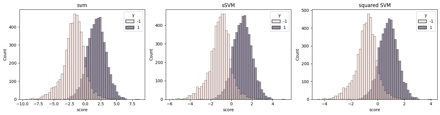
Compare SVM & Smooth SVM & Squared SVM

## print best results per loss
import pandas as pd
df = pd.DataFrame(grid_search.cv_results_)
df['Loss'] = df['param_clf__loss'].apply(lambda x: x['name'])
df = df.sort_values('mean_test_score', ascending=False)
best = df.drop_duplicates(subset=['Loss'])
table = best[['Loss', 'param_clf__C', 'mean_test_score']].rename(
    columns={'param_clf__C': 'Best C', 'mean_test_score': 'CV Score'}
)

print(table.to_string(index=False))

       Loss  Best C  CV Score
        svm     0.1    0.8922
       sSVM     0.1    0.8920
squared SVM     0.1    0.8913

## plot score distributions for best models
import seaborn as sns
import warnings
import matplotlib.pyplot as plt
warnings.filterwarnings("ignore", "is_categorical_dtype")
warnings.filterwarnings("ignore", "use_inf_as_na")

fig, axes = plt.subplots(1, 3, figsize=(15, 4))
for i in range(len(best)):
    loss = best['Loss'].iloc[i]
    c = best['param_clf__C'].iloc[i]

    pipe = Pipeline([
        ('scaler', StandardScaler()),
        ('clf', plq_Ridge_Classifier(loss={'name': loss}, C=c))
    ])
    pipe.fit(X, y)

    score = pipe.decision_function(X)
    df = pd.DataFrame({'score': score, 'y': y})
    sns.histplot(df, x="score", hue="y", ax=axes[i]).set_title(loss)

plt.tight_layout()
plt.show()