FairSVM¶

The FairSVM solves the following optimization problem:

\[\begin{split}\begin{aligned} \min_{\beta \in \mathbb{R}^d}\quad & \frac{C}{n}\sum_{i=1}^n (1-y_i\beta^\top x_i)_+ + \frac{1}{2}\|\beta\|_2^2, \\[1ex] \text{subject to}\quad & \frac{1}{n}\sum_{i=1}^n z_i\,\beta^\top x_i \le \rho,\quad \frac{1}{n}\sum_{i=1}^n z_i\,\beta^\top x_i \ge -\rho. \end{aligned}\end{split}\]

where:

\(x_i \in \mathbb{R}^d\) is a feature vector
\(y_i \in \{-1,1\}\) is a binary label
\(z_i\) is a collection of centered sensitive features, such as gender and/or race, satisfying

\[\sum_{i=1}^n z_{ij}=0\]
\(z_i \in \mathbb{R}^{d_0}\) is a \(d_0\)-length sensitive feature vector
\(\rho \in \mathbb{R}_+^{d_0}\) is a vector of constants that trade off predictive accuracy and fairness

The constraints limit the correlation between the sensitive features and the decision function, helping ensure fairness in predictions.

Note. Since the hinge loss is a plq function and the fairness constraints are linear, we can optimize this model using rehline.plq_Ridge_Classifier.

[1]:

## install rehline
%pip install rehline -q

[2]:

## simulate data
import numpy as np
from sklearn.datasets import make_classification
from sklearn.preprocessing import StandardScaler

scaler = StandardScaler()

n, d = 10000, 5
X, y = make_classification(n_samples=n, n_features=d, n_redundant=2, random_state=42)
y = 2 * y - 1
X = scaler.fit_transform(X)

## we take the first column of X as sensitive features, and tol is 0.1
sen_idx = [0]
tol_sen = 0.1

SVM as baseline¶

[3]:

## we first run a SVM
from rehline import plq_Ridge_Classifier

clf = plq_Ridge_Classifier(loss={"name": "svm"}, C=1.0, max_iter=50000)
clf.fit(X=X, y=y)

[3]:

plq_Ridge_Classifier(loss={'name': 'svm'}, max_iter=50000)

In a Jupyter environment, please rerun this cell to show the HTML representation or trust the notebook.
On GitHub, the HTML representation is unable to render, please try loading this page with nbviewer.org.

FairSVM¶

[4]:

## solve FairSVM via `plq_Ridge_Classifier` by adding `constraint`
import warnings

warnings.filterwarnings("ignore")
fclf = plq_Ridge_Classifier(
    loss={"name": "svm"}, constraint=[{"name": "fair", "sen_idx": sen_idx, "tol_sen": tol_sen}], C=1.0, max_iter=50000
)
fclf.fit(X=X, y=y)

[4]:

plq_Ridge_Classifier(constraint=[{'name': 'fair', 'sen_idx': [0],
                                  'tol_sen': 0.1}],
                     loss={'name': 'svm'}, max_iter=50000)

Results¶

[5]:

import pandas as pd

## sensitive features
X_sen = X[:, sen_idx]

## score
score = clf.decision_function(X)
fscore = fclf.decision_function(X)

svm_perf = len(y[score * y > 0]) / n
fsvm_perf = len(y[fscore * y > 0]) / n

svm_corr = score.dot(X_sen) / n
fsvm_corr = fscore.dot(X_sen) / n

# Create a pandas DataFrame to store the results
results = pd.DataFrame(
    {
        "Model": ["SVM", "FairSVM"],
        "Train Performance": [svm_perf, fsvm_perf],
        "Correlation with Sensitive Features": [svm_corr[0], fsvm_corr[0]],
    }
)

# Print the results as a table
print(results.to_string(index=False))

  Model  Train Performance  Correlation with Sensitive Features
    SVM             0.8927                             2.417714
FairSVM             0.5278                             0.100728

[6]:

import warnings

import matplotlib.pyplot as plt
import pandas as pd
import seaborn as sns

warnings.filterwarnings("ignore", "is_categorical_dtype")
warnings.filterwarnings("ignore", "use_inf_as_na")

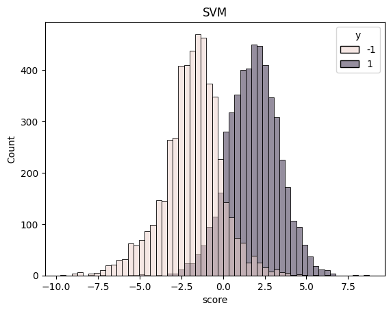
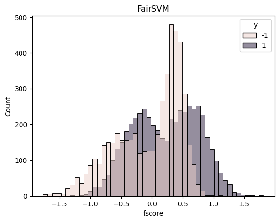
df = pd.DataFrame({"score": score, "fscore": fscore, "y": y})

sns.histplot(df, x="score", hue="y").set_title("SVM")
plt.show()
sns.histplot(df, x="fscore", hue="y").set_title("FairSVM")
plt.show()