Custom QR

The Custom QR solves the following optimization problem:

\[\min_{\mathbf{\beta} \in \mathbb{R}^d} C\sum_{i=1}^n \rho_{\kappa}(y_i-\mathbf{x}_i^\top\mathbf{\beta}) +\frac{1}{2}\|\mathbf{\beta}\|_2^2,\]

\[\text{subject to} \quad A\mathbf{\beta}+b \ge 0,\]

where:

• \(\mathbf{x}_i \in \mathbb{R}^d\) is a feature vector

• \(y_i \in \mathbb{R}\) is a continuous response variable

• \(\rho_{\kappa}(u)=u\big(\kappa-\mathbf{1}(u<0)\big)\) is the quantile (check) loss

• \(A \in \mathbb{R}^{K \times d}\) and \(b \in \mathbb{R}^{K}\) define custom linear constraints

The custom constraints allow arbitrary prior knowledge (e.g. sign, ordering, budget, or linear relation constraints) to be incorporated into quantile regression.

Note. Since the check loss is a plq function and the constraints are linear (\(A\beta+b\ge0\)), we can optimize it using rehline.plq_Ridge_Regressor.

## install rehline
%pip install rehline -q

## simulate data
from sklearn.datasets import make_regression
from sklearn.preprocessing import StandardScaler
import numpy as np

scaler = StandardScaler()

n, d = 10000, 5
X, y = make_regression(n_samples=n, n_features=d, noise=1.0, random_state=42)
X = scaler.fit_transform(X)
y = y / y.std()

# Example: beta_0 + beta_1 >= 3
A = np.zeros((1, d))
A[0, 0] = 1
A[0, 1] = 1
b = np.array([-3.0])

QR as baseline

## we first run a QR
from rehline import plq_Ridge_Regressor

clf = plq_Ridge_Regressor(
    loss={'name': 'QR', 'qt': 0.5},
    C=1.0,
    max_iter=10000,
    fit_intercept=False
)
clf.fit(X=X, y=y)

plq_Ridge_Regressor(fit_intercept=False, max_iter=10000)

In a Jupyter environment, please rerun this cell to show the HTML representation or trust the notebook.
On GitHub, the HTML representation is unable to render, please try loading this page with nbviewer.org.

Custom Constraint

## solve custom via `plq_Ridge_Regressor` by adding `constraint`
from rehline import plq_Ridge_Regressor

cclf = plq_Ridge_Regressor(
    loss={'name': 'QR', 'qt': 0.5},
    constraint=[{'name': 'custom', 'A': A, 'b': b}],
    C=1.0,
    max_iter=10000,
    fit_intercept=False
)
cclf.fit(X=X, y=y)

plq_Ridge_Regressor(constraint=[{'A': array([[1., 1., 0., 0., 0.]]),
                                 'b': array([-3.]), 'name': 'custom'}],
                    fit_intercept=False, max_iter=10000)

In a Jupyter environment, please rerun this cell to show the HTML representation or trust the notebook.
On GitHub, the HTML representation is unable to render, please try loading this page with nbviewer.org.

import pandas as pd
## score
score = clf.predict(X)
cscore = cclf.predict(X)

qr_perf = np.mean((y - score)**2)
cqr_perf = np.mean((y - cscore)**2)

# Create a pandas DataFrame to store the results
results = pd.DataFrame({
    'Model': ['QR', 'Custom QR'],
    'Train MSE': [qr_perf, cqr_perf]
})

# Print the results as a table
print(results.to_string(index=False))
#Print the results of custom constraint
lhs = cclf.coef_[0] + cclf.coef_[1]
print(f"\ncoef_0 + coef_1 = {lhs:.8f} >= 3: {lhs >= 3}")

    Model  Train MSE
       QR   0.000097
Custom QR   1.352705

coef_0 + coef_1 = 3.00000008 >= 3: True

import seaborn as sns
import pandas as pd
import warnings
import matplotlib.pyplot as plt
warnings.filterwarnings("ignore", "is_categorical_dtype")
warnings.filterwarnings("ignore", "use_inf_as_na")

n_sample = 50
X_sample, y_sample = X[:n_sample], y[:n_sample]
qr_sample = clf.predict(X_sample)
cqr_sample = cclf.predict(X_sample)

df = pd.DataFrame({
    'x0': X_sample[:, 0],
    'real_y': y_sample,
    'QR': qr_sample,
    'Custom_QR': cqr_sample
})

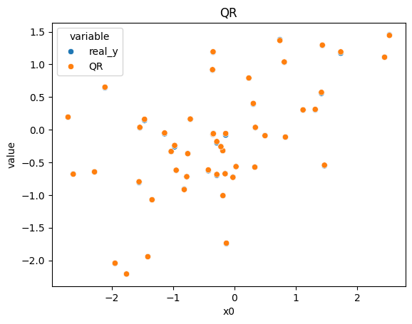
df1 = df[['x0', 'real_y', 'QR']].melt(id_vars='x0')
sns.scatterplot(data=df1, x='x0', y='value', hue='variable').set_title("QR")
plt.show()
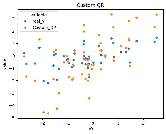
df2 = df[['x0', 'real_y', 'Custom_QR']].melt(id_vars='x0')
sns.scatterplot(data=df2, x='x0', y='value', hue='variable').set_title("Custom QR")
plt.show()